In the last post, we discussed how to modify the traffic path using summarization for external routes. Today we will continue discussing Traffic Engineering using OSPF summarization for intra-area routes. So, let’s get started.
Just to recap: The Inter-Area summarization is performed in ABRs, it summarizes Type-1 into Type-3 LSAs. We can perform OSPF traffic engineering with summarization when we have multiple exit points out of an area or multiple exit points out of the autonomous system using longer prefix match over shorter prefix match routing.
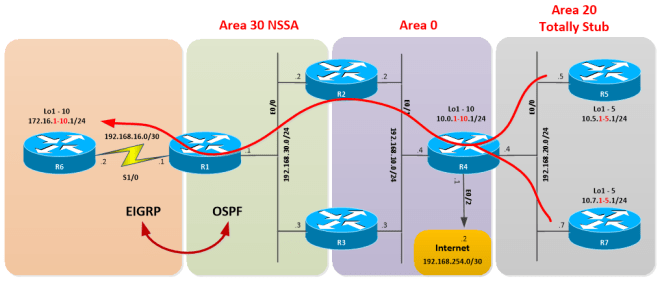
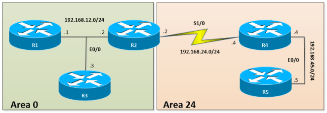
Let’s use the same topology we have been using so far but with a few changes:

Here you can download the diagram and configuration files: TE with OSPF Summarization – Part II
Among the changes done with respect to the topology used in the previous post, I can mention the creation and advertisement of 10 loopback interfaces in R1, the interface Lo0 in R1 is not being advertised into OSPF and the re-numbering of the loopback interfaces in R4. Another change is the ospf cost manually set to 20 in the Ethernet0/1 interface of R3.
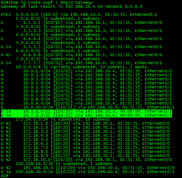
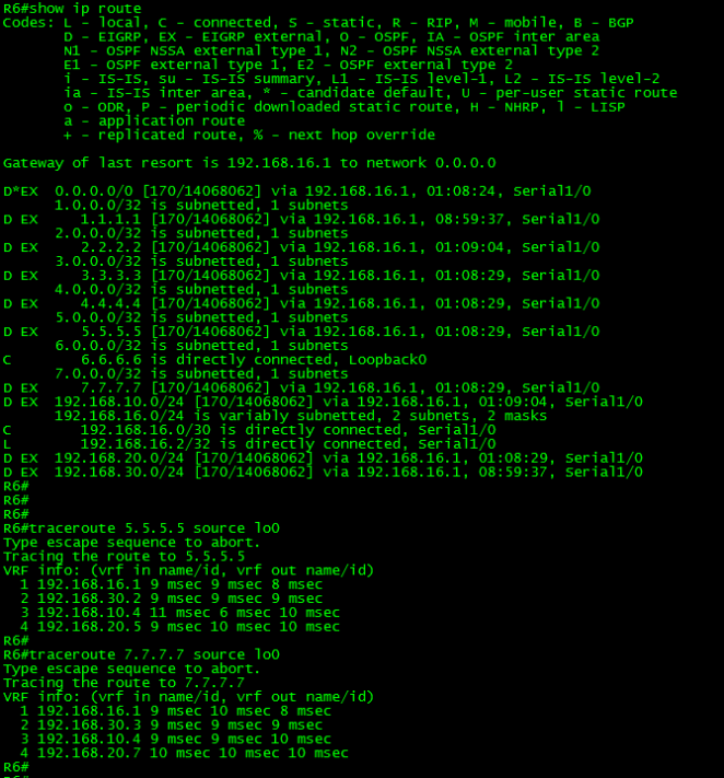
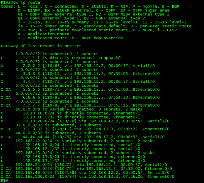
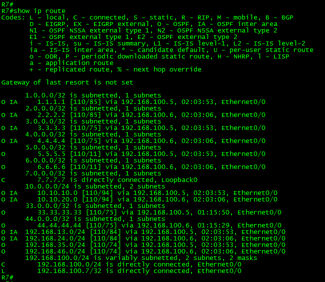
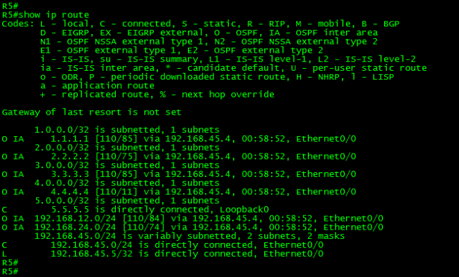
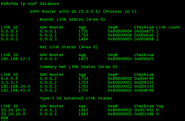
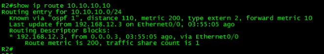
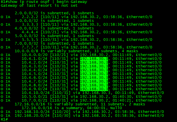
Let’s take a look to the routing table from the perspective of R1:

As can be seen in the above output, R1 is routing the eastbound traffic through R2. This is because of the higher OSPF cost assigned in the interface Ethernet0/1 of R3.
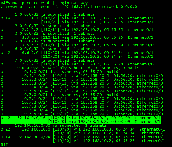
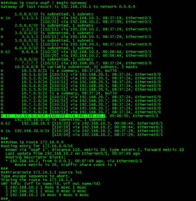
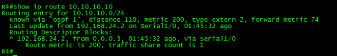
Now let’s take a look to the routing table from the perspective of R4:

From R4’s perspective, westbound traffic is load-balanced. So, let’s play a little bit with traffic engineering.
Goal 1:
Eastbound traffic from R1 destined to the loopback interfaces in R4 must go through R2.
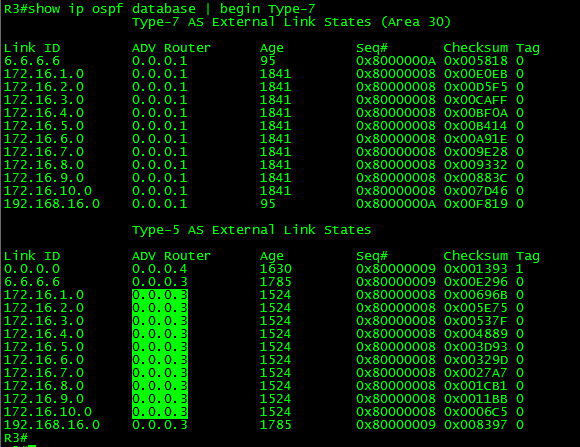
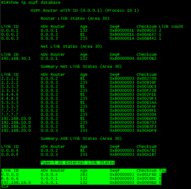
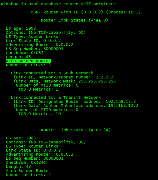
Let’s start by taking a look to the LSA corresponding to the loopbacks: (One loopback will be fine, the rest will have the same output.)

As shown in the output, both ABRs generated LSAs corresponding to the route 10.4.1.0/24; however only the route with best metric was installed in the routing table.
To achieve the goal, we will have to summarize the loopbacks in one of the ABRs and take advantage of longer prefix match over shorter prefix match routing. Because the goal dictates route through R3 we have to summarize the routes in the ABR R2, so let’s summarize the loopbacks into a /20 range which covers from 10.4.1.1 to 10.4.15.254.
In R2 (ABR):
!
router ospf 1
area 0 range 10.4.0.0 255.255.240.0
!
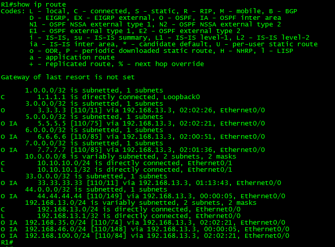
Now let’s take a look to the routing table in R1:
As can be seen in the above output, a summary route (10.4.0.0/20) was advertised from R2 and the more specific routes are now being advertised by R3.
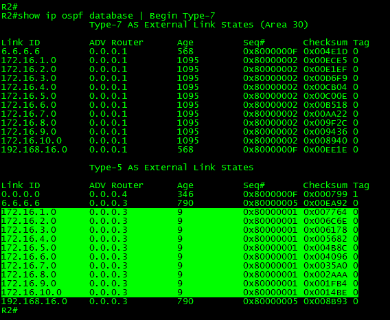
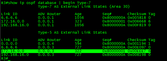
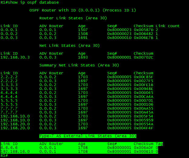
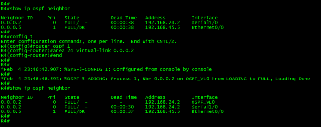
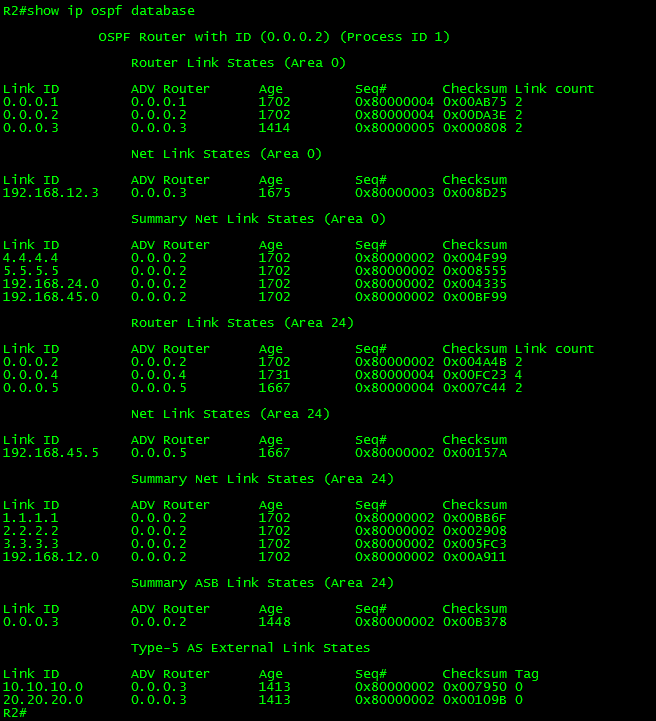
Let’s take a look at link-state database in R2, specifically Area 30:
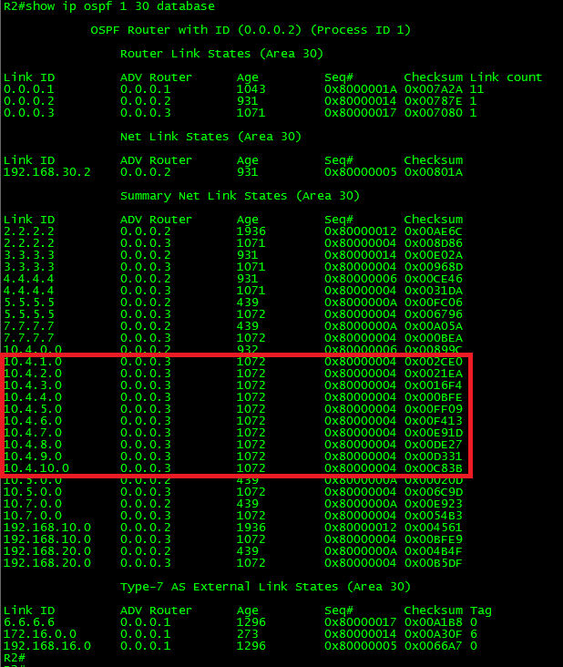
What happened here was that unlike R3, R2 ABR instead generating Type-3 LSAs for each loopback interface, it generates a single Type-3 summary LSA. Thus, R3 advertise more specific routes to R1.
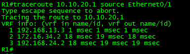
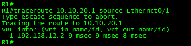
Finally, let’s test the solution tracing routes to the loopbacks and directions in R5 and R7.

As seen in the above output, the solution worked. The first trace sourced from Loopback1 in R1 route through R3 to reach Loopback1 in R4. The other traces route through R2 to reach the loopbacks in R5 and R7 respectively.
Let’s complicate a little bit more the traffic engineering examples.
Goal 2:
We have been requested to divide the westbound traffic from R1 towards R4 loopback interfaces into two summary addresses and route them as follows:
- The Summary Address 10.1.0.0/21 must be routed through R3.
- The Summary Address 10.1.8.0/21 must be routed through R2.
- In the routing table of R4, only the summarized ranges belonging to the loopback interfaces of R1 must be displayed.
So, let’s do it.
First, let’s take a look to the routing table from the perspective of R4:

As shown above, all of the westbound traffic is being load-balanced between R2 and R3 ABRs.
So, let’s proceed with the tasks:
Create the summary address 10.1.0.0/21 in R2 and the summary address 10.1.8.0/21 in R3.
In R2 (ABR):
!
router ospf 1
area 30 range 10.1.0.0 255.255.248.0
!
In R3 (ABR):
!
router ospf 1
area 30 range 10.1.8.0 255.255.248.0
!
Now let’s take a look to the routing table of R4:

Well, the summarization works as shown above. The traffic towards R1’s loopback interfaces is routed as requested. But the routing table also has more specific routes instead summaries. Also, note the routes for the external domain. The routes to 172.16.0.0/16 and 192.168.16.0/30 are now been advertised only via R3. But why?
Now we have two things to figure it out.
Let’s start with the summarization problem, and then we will see what happened to those routes.
For the summarization, we know that the more specific routes rule is working. Now we have to find the way to suppress them.
If we also apply summarization of the specific routes in each ABR we will have again load-balancing. Let’s make the change and take a look. Of course, we have to apply the same summarization applied to the ABRs in an inverse way. In other words, the summarization applied to R3 into R2 and vice versa.
In R2 (ABR):
!
router ospf 1
area 30 range 10.1.8.0 255.255.248.0
!
In R3 (ABR):
!
router ospf 1
area 30 range 10.1.0.0 255.255.248.0
!
After the changes were applied both ABRs will have summarization applied for both ranges in their routing process as follows:


Now, let’s take a look again to the routing table in R4:

Ok, the summary addresses are now being load-balanced, but wait a minute! Now we have again the routes to the External domain load-balanced. This means the change we just did is directly related. We will go back to this in a minute. Let’s finish the first problem.
As can be seen in the above output, the summary addresses are being load balanced because they have identical metric.
Now what we can do to change the traffic pattern is modify the metric to the summary addresses.
To do this, we will have to manually alter the cost on each ABR for the desired routes.
Let’s make the following change:
Because the summary Address 10.1.0.0/21 must be routed through R3, let’s modify the cost of the summary address in the ABR R2 and make it higher and let’s take a look at the result in the routing table of R4.
In R2 (ABR):
!
router ospf 1
area 30 range 10.1.0.0 255.255.248.0 cost 20
!

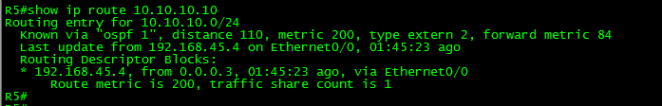
As shown in the above output, now the route 10.1.0.0/21 is now reachable only via R3.
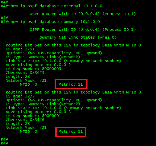
Now, let’s take a look at the summary Type-3 LSA:
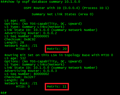
As can be seen, the metric of the LSA advertisement is now 20 when received from R2 and 11 when received from R3. Now, the lowest metric wins thus its installed in the RIB.
Now let’s do the change for the other summary route.
Because the summary Address 10.1.8.0/21 must be routed through R2, let’s modify the cost of the summary address in the ABR R3 and make it higher and let’s take a look at the result in the routing table of R4.
In R3 (ABR):
!
router ospf 1
area 30 range 10.1.8.0 255.255.248.0 cost 20
!

As shown in the above output, now the route 10.1.8.0/21 is now reachable only via R2.
Finally, the desired traffic pattern was achieved and the task was completed.
Now, let’s talk about the External routes. Why did they change when we applied the summarization? This behavior is clearly defined in the RFC 3101, in section 2.3. I would recommend you to read it.
Long story short: It has to be with the forwarding address, or better said: The way NSSA treat forward addresses when redistributing. The selection process to choose the forwarding address is: Choose the highest IP address of an internal address; if an internal address is not available, it will prefer the higher found OSPF stub network.
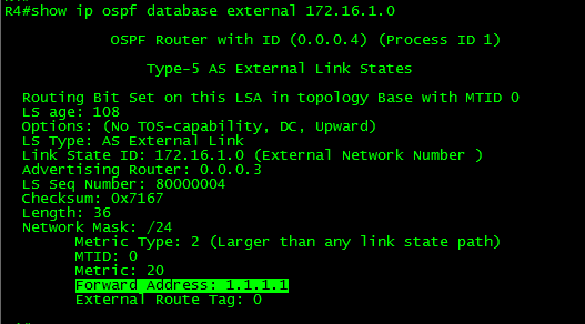
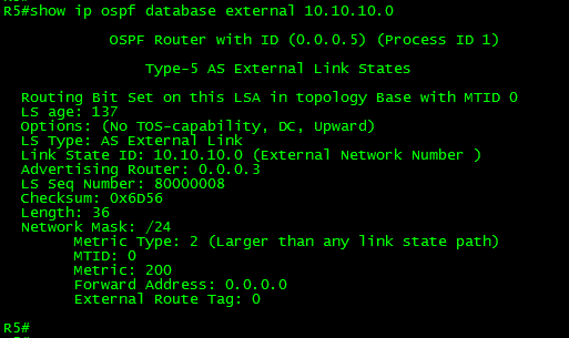
Let’s take a look to the external LSA:

In this case, the router has compared Loopback0 and Loopback1. Because Loopback1 has the higher IP address it wins.
The Forward Address (10.1.1.1) is within the range 10.1.0.0/21 previously summarized and routed throughout R3.
It is time to close this long post. In the next one, we will start discussing OSPF filtering.
Thank you for visiting.