Traffic Engineering with OSPF Summarization (Part 1)

In today’s posts, we will start discussing the additional applications also provided by OSPF summarization. OSPF summarization can be also used for Traffic Engineering and Filtering.

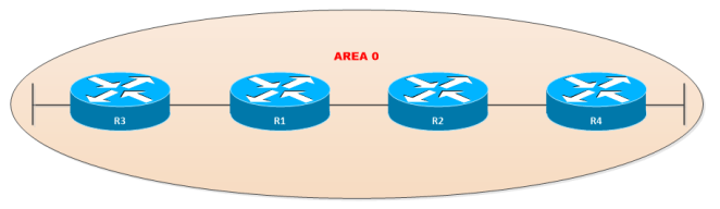
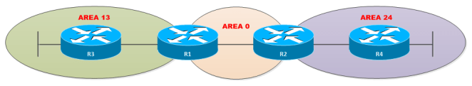
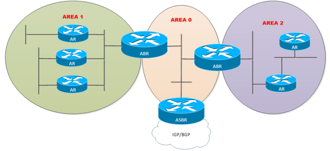
Just to recap:   OSPF scalability is achieved by summarization of the topology using OSPF areas and network prefixes summarization.   Now, OSPF summarization can only be applied for inter-area and external routes.      The Inter-Area summarization is performed in ABRs, it summarizes Type-1 into Type-3 LSAs.    The external routes summarization is performed on ASBRs, it summarizes Type-5 into Summarized Type-5 LSAs and type-7 into Summarized Type-7 LSAs.

When summarization is done, the discard route (route to Null0) is automatically created.   This is a loop prevention mechanism used to discard routes if no more specific route to a network destination exists.   In OSPF, summarization must be done in a manual way.    Please take a look at the previous post for details in OSPF summarization and its configuration.

Using OSPF summarization for Traffic Engineering:

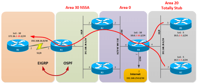
We can perform OSPF traffic engineering with summarization when we have multiple exit points out of an area or multiple exit points out of the autonomous system.    It is achieved using longer prefix match over shorter prefix match routing.     In other words, route traffic over more specific routes than summary routes.     Let’s use the following topology to illustrate how traffic engineering with summarization works:

OSPF-SUMMARY-APPS-01

Here you can download the diagram and configuration files: TE with OSPF Summarization – Part I.

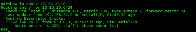
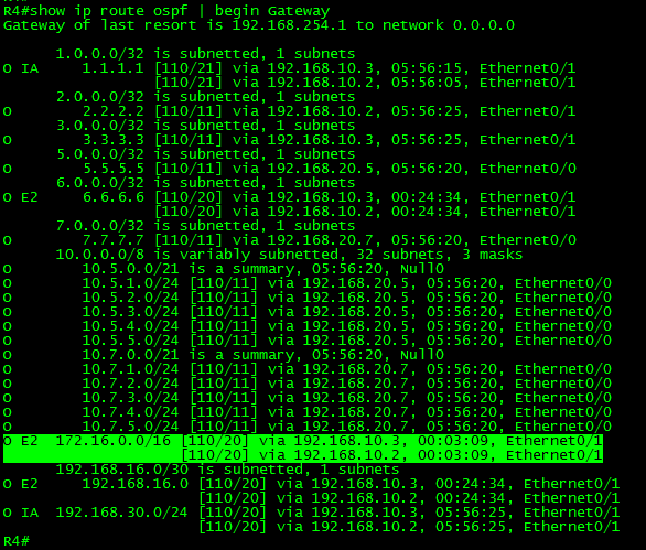
Let’s take a look to the routing table in R4:

OSPF-SUMMARY-APPS-02

As can be seen in the above output, R4 (ABR for area 20) has inter-area routes (Red) coming from R5 and R7 belonging to area 20 respectively with its corresponding /21 summary discard routes pointing to Null0.

OSPF-SUMMARY-APPS-03

R4 also has external routes (Above in Blue) coming from R6 (EIGRP Domain) as shown below.

OSPF-SUMMARY-APPS-04

Now, the external routes are been load-balanced between R2 and R3 ABRs.  Let’s take a look to the LSA corresponding to the prefix 172.16.1.0.

OSPF-SUMMARY-APPS-05

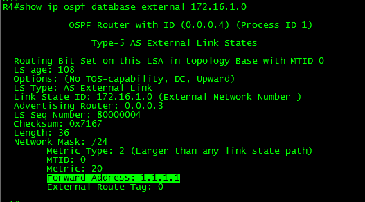
The LSA corresponds to a Type-5 External LSA, the Advertising Router is R3 (RID 0.0.0.3).  This field corresponds in this case to the “Elected Translator Router”, or the router in charge to translate from Type-7 LSA into Type-5 LSA, however, the route comes from R1 (LINK ID 1.1.1.1) which is the router doing the redistribution into OSPF.    Now let’s take a look to the LSA corresponding to the link-ID 1.1.1.1:

OSPF-SUMMARY-APPS-06

As can be seen in the output, the Type-3 LSAs corresponding to the link-id 1.1.1.1 has two possible routes.   From R2 (Advertising Router: 0.0.0.2) and R3 (Advertising Router: 0.0.0.3) with identical metric.   Thus, the route is been load-balanced.

Now, with this information let’s do some traffic Engineering:

Goal:

Traffic from the networks 10.0.0.0/21 in R4 (Area 0) and the whole Area 20 must use R2 to reach the 172.16.0.0/16 networks in the EIGRP domain.

OSPF-SUMMARY-APPS-07

At first hand we know the Totally Stubby Area 20 will automatically generate a default route, it will have into its link-state database Type-1 and Type-2 LSAs containing intra-area information and a Type-3 Summary LSA with the default route pointing to R4, which is the only way out to reach other areas and external routes.    This is the case for R5 and R7 respectively as shown below:  (Only R5 information shown by brevity)

OSPF-SUMMARY-APPS-08

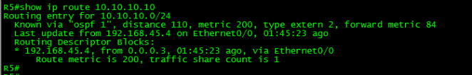
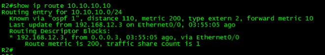
We also know the routes to the external EIGRP domain are being load-balanced between R2 and R3 in R4:

OSPF-SUMMARY-APPS-09

So, let’s apply the Summarization in the ASBR (R1) and examine the routing table in R4 again:

In R1 (ASBR):

!
router ospf 1
summary-address 172.16.0.0 255.255.0.0
!

OSPF-SUMMARY-APPS-10

As shown in the above output, the routing table of R4 now has a summary 172.16.0.0/16 route; the route is still load-balanced.    The requirement is to route the traffic to the external EIGRP domain via R2.   Here is where the tricky part comes.

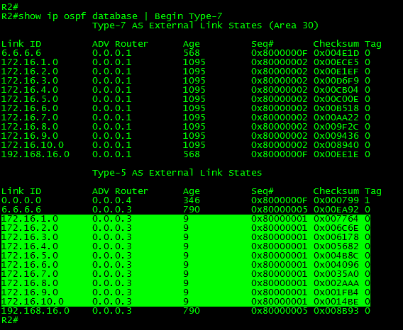
Let’s take a look at the link-state databases in R2 and R3, in particular to the Type-5 and Type-7 LSAs.

OSPF-SUMMARY-APPS-11

OSPF-SUMMARY-APPS-12

As can be seen, the ABRs translated Type-7 into Summarized Type-7 LSAs and as expected a Type-5 summary LSA was generated by the elected Type-7 to Type-5 Translator Router.  In this case R3 (RID 0.0.0.3).   R4 will receive only the Summarized Type-5 LSA;  Type-7 LSAs are not allowed out of NSSA areas, the ABR connecting NSSA areas will generate a Type-5 LSA to advertise the external routes on behalf of the ASBR.

But, what can we do to route the traffic only from R2?    Currently, we have two identical paths with identical metric.   Let’s recap and change the approach.   For traffic engineering with OSPF summarization to work is needed a summary route in one of the ABRs and more specific routes in the other.  So, let’s undo the previous change and summarize in the one of the ABRs.

In R1 (ASBR):

!
router ospf 1
no summary-address 172.16.0.0 255.255.0.0
!

In theory, if we summarize the loopbacks of R6 (EIGRP Domain) into 172.16.0.0/16 in R3, the more specific routes in R2 will be preferred.   Let’s give it a try.

In R3 (ABR):

!
router ospf 1
summary-address 172.16.0.0 255.255.0.0
!

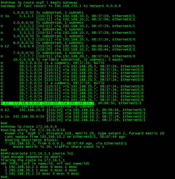
Now let’s take a look to the routing table in R4:

OSPF-SUMMARY-APPS-13

Wait a minute.  It didn’t work!    Let’s find out why?

Let’s take a look again to the link-state databases in the ABRs, in particular to the Type-5 and Type-7 LSAs.

OSPF-SUMMARY-APPS-14

OSPF-SUMMARY-APPS-15

As can be seen in the above output, both ABRs have Type-7 LSAs flooded in the NSSA area from the ASBR (R1).  They also have a Type-5 LSA corresponding to the summarized prefix 172.16.0.0/16, but it’s not supposed to have in R2 Type-5 LSAs with specific routes?  Something likes the following:

OSPF-SUMMARY-APPS-16

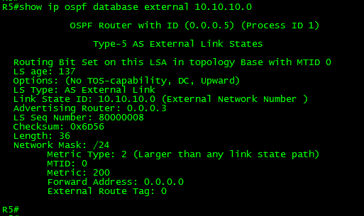
Well, let’s take a closer look to the external LSA in R2:

OSPF-SUMMARY-APPS-17

Have you noticed the problem?   The forwarding address of the Type-5 LSA is set to null (0.0.0.0).  This means that the route is reachable only via the advertising router.   You may be thinking that the advertising router is the ASBR (R1) and this is correct in part, but you have to remember when multiple ABRs are present only one is elected as the Type-7/Type-5 translator.

The ABR R3 was elected translator because it has higher Router-ID (RID) configured.  R3 has suppressed the most specific prefixes and replace them with a single Summarized Type-5 LSA and then it flooded to all routers within the area.

The way to solve this task is to apply the summarization in R2 and make it the Type-7 to Type-5 router translator.    As you may know, the election is “automatic”, this means that changing the RID in R2 to something higher it will change the role to the Type-7/Type-5 translator.   But, it is also required when changing the RID in an OSPF-enabled router clearing the process.   Clearing the OSPF process is a disruptive change, so plan accordingly if you choose this path.

Another way to do this it’s instructing the ABR R2 to become always the Type-7/Type-5 translator.  This is done in the nssa area definition, adding the keywords translate type 7 always.   This change is non-disruptive.

Let’s make the change and give it a try.

In R2 (ABR):

!
router ospf 1
area 30 nssa translate type7 always
summary-address 172.16.0.0 255.255.0.0
!

OSPF-SUMMARY-APPS-18

OSPF-SUMMARY-APPS-19


As seen in the above outputs, the goal was achieved.   Traffic from the loopbacks in R4 and networks in Area 20 now traverses R2 as the primary path to reach the EIGRP domain.    Also, redundancy is in place. If a failure occurs in R2, then R3 will advertise the summary route.

It is time to close this long post.  In the next one, we will discuss traffic engineering with inter-area summarization.   Thank you for visiting.

Interconnecting OSPF Areas – Virtual Links

In a multi-area OSPF network, all areas must be connected to the backbone area Zero (0), otherwise, no inter-area communications are possible.

Virtual-Links are OSPF tunnel interfaces used to solve situations where is necessary connecting a nonzero area to the backbone using another nonzero area as transit.

Let’s use the following example to illustrate the problem:

OSPF-CONN-VL1

Relevant Configuration:

R1:

!
interface Loopback0
ip address 1.1.1.1 255.255.255.255
ip ospf 1 area 0
!
interface Ethernet0/0
ip address 192.168.12.1 255.255.255.0
ip ospf 1 area 0
!
router ospf 1
router-id 0.0.0.1
!

R2:

!
interface Loopback0
ip address 2.2.2.2 255.255.255.255
ip ospf 1 area 0
!
interface Ethernet0/0
ip address 192.168.12.2 255.255.255.0
ip ospf 1 area 0
!
interface Serial1/0
ip address 192.168.24.2 255.255.255.0
ip ospf 1 area 24
!
router ospf 1
router-id 0.0.0.2
!

R3:

!
interface Loopback0
ip address 3.3.3.3 255.255.255.255
ip ospf 1 area 0
!
interface Ethernet0/0
ip address 192.168.12.3 255.255.255.0
ip ospf 1 area 0
!
router ospf 1
router-id 0.0.0.3
!

R4:

!
interface Loopback0
ip address 4.4.4.4 255.255.255.255
ip ospf 1 area 45
!
interface Ethernet0/0
ip address 192.168.45.4 255.255.255.0
ip ospf 1 area 45
!
interface Serial1/0
ip address 192.168.24.4 255.255.255.0
ip ospf 1 area 24
!
router ospf 1
router-id 0.0.0.4
!

R5:

!
interface Loopback0
ip address 5.5.5.5 255.255.255.255
ip ospf 1 area 24
!
interface Ethernet0/0
ip address 192.168.45.5 255.255.255.0
ip ospf 1 area 45
!
router ospf 1
router-id 0.0.0.5
!

As can be seen from the diagram, R2 and R4 have interfaces in multiple areas. R2 has an interface in Area 0 (backbone) and another interface in Area 24. R4 has an interface in Area 24 and another interface in area 45.

You might think that R2 and R4 are ABRs. However in Cisco deployments, for a router becomes ABR requires that at least one interface is connected to area 0 (backbone).

Now let’s take a look at the routing tables of R1 and R5 respectively.


As can be seen in the above outputs, R1 has OSPF routes of the loopback interfaces of R2, R3, and R4 and also has the route of the segment 192.168.24.0/24 which connects R2 and R4.  However, the route of the segment 192.168.45.0/24 and the loopback of R5 are missing.   In R5 only the connected routes are present.

Now let’s question R1 and R5 about their known ABRs.

According to the above outputs, R1 identifies R2 as the only ABR in OSPF.  R5 can’t identify any.

Remember, when a Router turns into an ABR what it does is set the “b” bit into its Type-1 LSA, then generates and flood Type-3 LSAS.    The flooding scope of Type-3 LSA is a single area.

So, let’s take a look to R2 and R4 Type-1 LSAs and see if the b-bit is set.  We know R2 has it.  R1 already identifies R1 as ABR, but I want to show you the difference between them.

As expected, R2 has the “b” bit set and is claiming to be and ABR while R4 is not.   This is the reason why the routes are not been propagated.   In order that R4 become an ABR, it is necessary that one of its interfaces to be connected to the backbone area.

There are many ways to solve this problem.  For example we can try renumbering the Area 45 and make a single area 24. Or we can just connect an interface between R2 and R5 as part of area 45. But what if none of these solutions are possible?  What if the devices don’t have free interfaces or they are placed too far from each other?   What if renumbering the area is not allowed?

Well, in this case we can use OSPF virtual-links or GRE tunnels.   In my humble opinion, it is better to use Virtual-Links instead of GRE.   To start, GRE is process-switched.  GRE also adds encapsulation overhead.  GRE encapsulates data traffic and routing traffic unlike Virtual-links, where only the routing updates are tunneled.   The only advantage of GRE over Virtual-Links is that supports tunnels through stub areas.   So let’s try using virtual-links and in a following post I will explain how to use GRE.

Let’s take a look to the requirements to configure the virtual-link:

  • The transit area cannot be a stub area.
  • The transit area shouldn’t have filtering.
  • The transit area must have full routing information.

Looking at the configuration files exposed before, note that Area 24 is a normal area and there is no filtering applied.  The last thing we need to verify is the transit area routing information.  If it has full routing information then using a virtual-link is possible.   Let’s take a look to the routing table of R4 to verify this.

OSPF-CONN-VL-07

As can be seen in the above output, R4 which is the router connecting has full routing information.  This means that Area 24 can be used as transit.

Let’s move on the configuration:

To configure the OSPF virtual-link, use the command area {transit-area-id} virtual-link {destination-router-id}.   This command goes in the OSPF process definition both routers forming part of the transit area (R2 and R4).

OSPF-CONN-VL2


R2: 

!
router ospf 1
area 24 virtual-link 0.0.0.4
!

R4:

!
router ospf 1
area 24 virtual-link 0.0.0.2
!

OSPF-CONN-VL-08

After the configuration was done, a new adjacency was formed via interface OSPF_VL0.

This “interface” is as a matter of fact is a multi-hop point-to-point unicast adjacency; it is in essence an extension of Area 0 across the transit area.

Let’s take a look to the virtual link using the command show ip ospf virtual-links.

OSPF-CONN-VL-09

As can be seen in the above output, the virtual-link is a demand circuit.   This is a legacy concept coming from back on the day where dialup or ISDN circuits were in use.  Back then the customers pay the link depending on the connect time or usage.   Also note the Hello is suppressed and the DoNotAge LSA is allowed.   This means that once the virtual link is up, no hellos are exchanged and the normal LSU refresh (every 30 minutes) won’t take place.  These things must be taken into account when doing troubleshooting.   In some cases is necessary clearing the ospf process for the changes take place.

Let’s take a look to the link-state Database.

OSPF-CONN-VL-09-1

The above output show the DNA (DoNotAge) bit set in some LSAs.    Also note that R4 now show Type-1 LSAs from Area 0.

Let’s take a look of the self-originated Type-1 LSA of R4.

OSPF-CONN-VL-10

As can be seen on the above output, now R4 is setting the “b” bit to its Type-1 LSAs.  This means that R4 has turn into an ABR.

Finally let’s take a look to the routing table of R5:

OSPF-CONN-VL-11

Now R5 has full reachability to the network via the transit area.

It is time to close this long post. Thank you for visiting.

Interconnecting OSPF Areas

In a previous post, we learned how to configure OSPF within a single area. Now it is time to consider what would happen if this single area grows to let’s say, hundreds of routers?

Well, with such large number of routers and segments; the network changes are inevitable.   Having this in mind, we can anticipate some problems like frequent calculations of the shortest path first (SPF) algorithm, large link-state database and of course, a large routing table.  In order to avoid these issues, OSPF allows large areas can be separated into smaller ones.  This is also known as hierarchical routing.

Before go deep into this topic we have to recall the different OSPF router types:

  • Internal Router – Routers that have all interfaces in the same area.
  • Backbone Router – Routers where at least one OSPF interface must belong to area 0 (backbone area).
  • Area Border Router (ABR) – In Cisco IOS are the Routers that have at least one OSPF interface connected to Area 0 and at least one OSPF interface belong to a non-backbone area. This may not be the case for different platforms where the only requirement is having the interfaces in different areas regardless if they are connected to the backbone area or not.   IPEXPERT’s blog has an interesting post about this here.
  • Autonomous System Boundary Router (ASBR) – Routers injecting routes (Redistribution) from another routing protocol.

Let’s take a look at the following example:

OSPF-CONN-ABR

Relevant Configuration:

R1:

!
interface Loopback0
ip address 1.1.1.1 255.255.255.255
ip ospf 1 area 0
!
interface Ethernet0/0
ip address 192.168.12.1 255.255.255.0
ip ospf 1 area 0
!
router ospf 1
router-id 0.0.0.1
!

R2:

!
interface Loopback0
ip address 2.2.2.2 255.255.255.255
ip ospf 1 area 0
!
interface Ethernet0/0
ip address 192.168.12.2 255.255.255.0
ip ospf 1 area 0
!
interface Serial1/0
ip address 192.168.24.2 255.255.255.0
ip ospf 1 area 24
!
router ospf 1
router-id 0.0.0.2
!

R3:

!
interface Loopback0
ip address 3.3.3.3 255.255.255.255
ip ospf 1 area 0
!
interface Ethernet0/0
ip address 192.168.12.3 255.255.255.0
ip ospf 1 area 0
!
router ospf 1
router-id 0.0.0.3
!

R4:

!
interface Loopback0
ip address 4.4.4.4 255.255.255.255
ip ospf 1 area 24
!
interface Ethernet0/0
ip address 192.168.45.4 255.255.255.0
ip ospf 1 area 24
!
interface Serial1/0
ip address 192.168.24.4 255.255.255.0
ip ospf 1 area 24
!
router ospf 1
router-id 0.0.0.4
!

R5:

!
interface Loopback0
ip address 5.5.5.5 255.255.255.255
ip ospf 1 area 24
!
interface Ethernet0/0
ip address 192.168.45.5 255.255.255.0
ip ospf 1 area 24
!
router ospf 1
router-id 0.0.0.5
!

Area Border Router

As mentioned earlier, ABR’s are used to connect non-backbone areas to Area 0.  ABRs take the information contained in Type-1 and Type-2 and summarize it into Area 0.  In the above example, R1, R2, and R3 are backbone routers.  R2 is also acting as ABR between Area 0 and Area 24 respectively.   R4 and R5 are internal routers of Area 24.   R2 advertise itself as ABR by setting the “B” bit in its type 1 LSA.

OSPF-CONN-01

The above output displays the self-originated Type-1 (Router) LSA with the “B” bit set.  This is the ABR in the current topology.   Another way to identify ABRs is using the command show ip ospf border-routers.

OSPF-CONN-02

The above output displays the list of known ABRs from the perspective of R1.

Also, we have to keep in mind that an ABR keeps multiple copies of the link-state database, one for each area to which that router is connected.    ABRs create and flood Type-3 (Summary) LSAs within areas; it will generate more than one summary LSA if the address cannot be properly aggregated by a single prefix (i.e. Host Routes or loopbacks).

OSPF-CONN-03

As can be seen in the above output, R2 (ABR) has 2 copies of the link-state database.  The Type-3 Summary LSA information of Area 0 details 2 networks (192.168.24.0/24 and 192.168.45.0) and 2 host routes (4.4.4.4 and 5.5.5.5) belonging to the loopbacks of R4 and R5 while the Summary LSA of Area 24 details a single network (192.168.12.0/24) and 3 host routes (1.1.1.1, 2.2.2.2 and 3.3.3.3) belonging to the loopbacks of R1, R2 and R3 respectively.     In other words, the ABR is actually hiding the topology information within areas.

Now, let’s take a look to the routing table of R1 and see how to reach R5’s loopback:

OSPF-CONN-04

As can be seen in the above output, the routing table shows the routes belonging to area 24 as “O IA” meaning inter-area routing.  The intra-area routes of Area 0 are shown as “O”.   Another important thing to denote is the actual route to the loopback 0 of R5.    As you can see, the metric to reach 5.5.5.5 is 85 from R5.   This is because the metric is additive in this case.  It is the sum of the cost to reach the loopback of R5 from R1.  (R1—10—R2—64—R4—10—R5—1—Lo0 = 85).   The route describes the next hop:  “192.168.12.2, from 0.0.0.2”, which is the next-hop IP address and the Router-ID of R2.  R2 is the advertising the route on behalf of R5, not an IP address.

Now let’s take a look at R2’s information for the same route.

OSPF-CONN-05

Note the difference between the above output and the previous one.  Here we can see the route to 5.5.5.5 shown as “O” intra-area.   This is because R2 has the interface Serial1/0 in area 24; this makes the route internal for it.     From R2, the metric has also decreased to 75.  The route describes the next hop:  “192.168.24.4, from 0.0.0.5”, which is the next-hop IP address of R4 and the Router-ID of R5 which is advertising router.

Let’s take a look at R4’s information for the same route.

OSPF-CONN-06

As can be seen in the above output, the routing table shows the routes belonging to area 0 as “O IA” meaning inter-area routing.  The route to 5.5.5.5 is an intra-area route OSPF.  As expected, the metric has decreased to 11.  The route describes the next hop: “192.168.45.5, from 0.0.0.5”, which is the next-hop IP and the Router-ID of R5.

Finally in R5, ospf advertise the loopback 0 with Cost of 1.

OSPF-CONN-07

ABRs also create and flood Type-4 (ASBR Summary) LSAs when an ASBR is present.  This LSA is used to let other areas know where the ASBR is.

Autonomous System Boundary Router

ASBRs are routers injecting routes from another routing protocol or autonomous system.  The injection is done via Redistribution.   ABRs generate and flood Type-5 LSAs.

To inject routes into the OSPF domain, use the redistribute {connected|static|protocol}{metric <0-16777214>} {metric-type <1|2>} {subnets} {route-map} {tag <0-4294967295>} OSPF process command.

  • The {connected|static|protocol} statement is self-explanatory. It defines the source of the routes to be redistributed.
  • The {metric} keyword set the Cost of the route to be advertised. If the metric is not specified, OSPF will use a default value of 20 when redistributing routes from all IGPs.  When redistributing from BGP, the metric will be 1 by default.
  • The {metric-type} keyword forces the routes to be advertised as External Type 1 or Type 2. By default, Type 2 is used.   For more information about the route Types and LSA Types, please see the post OSPF LSA Flooding Scope.
  • The {subnets} keyword is required when redistributing subnetted networks. Without this keyword, only major networks will be redistributed.
  • The {route-map} keyword is an enhancement to the redistribution process. It allows using different policies for redistribution.
  • The {tag} keyword as its name implies, set a numeric tag value to the routes to be redistributed. This is widely used to control redistribution between protocols.

More on {route-maps} and {tags} in future posts.

For example, let’s use the same topology but we will configure R3 as ASBR:

OSPF-CONN-ABR-ASBR

In R3 we will make the following changes:

First, we will add two loopback interfaces and configure RIP:

!
interface Loopback10
ip address 10.10.10.10 255.255.255.0
!
interface Loopback20
ip address 20.20.20.20 255.255.255.0
!
router rip
version 2
network 10.0.0.0
network 20.0.0.0
no auto-summary
!

Finally, we will redistribute RIP into OSPF:


!
router ospf 1
redistribute rip metric 200 subnets
!

After redistribution was configured, R3 advertise itself as ASBR by setting the “E” bit in its type 1 LSA.

OSPF-CONN-07-1

The above output displays the self-originated Type-1 (Router) LSA with the “E” bit set.  This is the ASBR in the current topology.   Another way to identify ASBRs is using the command show ip ospf border-routers.

OSPF-CONN-07-2

Now let’s take a look at the link-state Database of R1 and its routing table.

OSPF-CONN-08

OSPF-CONN-09

As can be seen in the above output, R1 only has Type-1, Type2, Type-3 and Type-5 LSAs in their databases.  R1 and R3 have identical link-state Databases.  The routes to reach the RIP routes are “O E2” OSPF external routes Type 2.

Now, R2 is an ABR and contains identical database information as R1 and R3 for area 0.  R2 also has a database for area 24.

OSPF-CONN-10

The database of R2 for Area 24 contains Type-1, Type-2, Type-3, Type-4 and Type-5 LSAs.  As mentioned before, Type-4 LSAs are used to inform other areas where the ASBR is located.  It is used basically to provide reachability information for the ASBR.

R4 and R5 are internal routers of Area 24; they share the same database information.  For brevity, let’s focus in R5.

OSPF-CONN-11

OSPF-CONN-12

As expected, the link-state Database contains Type-1, Type-2, Type-3, Type-4 and Type-5 LSAs and the routing table show the routes as “O E2” OSPF External routes type 2.

Finally, let’s try to reach the IP address 10.10.10.10 from R5.

Let’s get started looking for the route itself:

OSPF-CONN-13

As you can see, the route is known by OSPF, the reported metric of the route is 200.  We have defined this metric when redistributing the route.  The route is External Type-2.  This is the advertised cost from the ASBR to the external destination network.   The forward metric is 84.   This metric is the total cost to the ASBR from R5.

The route describes the next hop: “192.168.45.4, from 0.0.0.3”, which is the IP address of R4 and the Router-ID of the advertising router R3 (ASBR).

Now let’s check R4 and R2:

OSPF-CONN-14

OSPF-CONN-15

As can be seen in the above outputs, the only change is metric and the next-hop to reach the advertising router.

OSPF-CONN-16

The advertising router remains the same because the forwarding address in the Type-5 LSA is set to 0.0.0.0 (null).   This means that the route is reachable only via the advertising router.

It is time to close this long post. Thank you for visiting.


OSPF Areas and Area Types

OSPF provides two levels of hierarchy through the use of Areas.  An easy way to explain what an Area is would be:  An OSPF area is a logical segment or a sub-domain containing networks, routers and links sharing the same area id.

Using multiple areas in OSPF reduces the router resource utilization because the routers belonging to the same area only maintain the network topology of the area where they belong. Thus, less LSA has to be flooded and maintained.  In other words, the Routers in other areas; don’t have information about the topology outside its own area.

An area is a 32-bit number which can be represented the same way as an IP address such  “area 0.0.0.0” or as a decimal number, such as “Area 0”.

OSPF-AT-Single-Area

The Area 0 is the backbone area in an OSPF domain.   If more than one area is configured, then Area 0 is required to provide inter-area communications.   This means that in an OSPF autonomous system, all areas must be physically connected to the backbone area 0.

OSPF-AT-Multi-Area

I’ve mentioned that all areas must be connected to Area 0; But, what about areas that cannot be physically connected to the area 0?

OSPF provides a native solution for this problem, OSPF Virtual-Links.  I will dedicate an entire post for this technology later on.

OSPF-AT-Virtual-Link.PNG

The Routers contained within the same area are called Area Routers (AR), the routers with a link in Area Zero (0) and a Non-Zero area is called Area Border Routers (ABRs).  Finally, the Routers with a link in Area Zero (0) or a Non-Zero area and redistributing from another Routing Protocol are called Autonomous System Boundary Routers (ASBRs).   Summarization can be done only on ABRs and ASBRs.

OSPF-Router-Type

OSPF Area Types

The OSPF area types can be divided into the following types:

  • Normal Areas
    • Standard.
    • Transit.
  • Stub Area.
    • Totally Stubby Area.
  • Not-So-Stubby Area (NSSA).
    • Totally NSSA.

Normal Area

Normal Areas can be standard or transit (backbone) areas.

  • The Standard areas are the non-zero defined areas where LSAs Type-1, 2, 3, 4 and 5 are allowed; this means that can accept intra-area, inter-area, and external routes.
  • The backbone area is, in essence, a Standard area but is the area from which all other areas in OSPF must be connected.

I’ve mentioned that summarization is possible only on ABRs and ASBRs; But, what about the default route?    Well I think is necessary to explain about the default-route in normal areas.

It is allowed to generate the default route in Normal Areas.  The default route is injected as Type-5 LSA.

In order to generate the default route use the default-information originate process command.  If the default route is not present in the Routing Table then won’t be generated unless the [always] keyword is added at the end of the command.

OSPF-AREA-Normal


Stub Area

Stub areas are typically used where the access to the rest of the network through a single link.  For these type of networks is not necessary having and maintaining a full link state database.   This area type can only accept intra-area, inter-area and the default route (generated by default).

Stub areas allow only LSAs Type-1, 2 and 3.   Redistribution is not allowed in Stub Areas.

The default route in a Stub area is generated by default and is injected in the area as Type-3 LSA.

To configure a Stub Area use the Area [x] stub process command.  This command must be added to the routers belonging to the stub area and also, must be added to the ABR connecting the stub area.

OSPF-AREA-STUB


Totally Stubby Area

Totally Stubby areas are an extension of Stub Areas and are in fact, the most restricted type of OSPF area.

In Totally Stubby Areas, the Routers receive only a default route from the ABRs, no External or Summary routes are allowed except for the default-route.   The default route in Totally Stubby area is generated by default and is injected in the area as Type-3 LSA.

To configure a Totally Stubby Area use the Area [x] stub no-summary process command.  This command with the no-summary keyword is required only on the ABR connecting the area.

The router connecting to the ABR does not require the no-summary keyword but requires to be defined as a stub.

OSPF-AREA-T-STUB

Not-So-Stubby Areas (NSSA)

Not-So-Stubby areas are also an extension of the stub areas.  This type of area adds the flexibility of redistribution of external routes into the area while retaining its stub characteristic.   This area type can only accept intra-area, inter-area, external and the default route (which is not generated by default).   Not-So-Stubby areas allow only LSAs Type-1, 2, 3 and 7.

When the default route in an NSSA is generated, it is injected in the area as Type-7 LSA.

To configure an NSSA use the Area [x] nssa [default-information-originate] process command.  This command must be added to the routers belonging to the NSSA area and must be also added to the ABR connecting the NSSA.  The default-information-originate keyword generates the default-route in NSSA.

OSPF-AREA-NSSA


Totally Stubby NSSA

Totally Stubby NSSA is an extension to the NSSA.  As a matter of fact, this is the most recommended form of NSSA area type.  This type of area adds the flexibility of redistribution of external routes into the area while retaining it’s totally stubbed characteristic.   This area type can only accept intra-area, external and the default route (which is generated by default).   Totally Stubby NSSA areas allow only LSAs Type-1, 2, [3] and 7.      The default route in a Stub area is generated by default and is injected in the area as Type-3 LSA.

To configure a Totally Stubby NSSA use the Area [x] nssa no-summary process command.  This command with the no-summary keyword is required only on the ABR connecting the area.

The router connecting to the ABR does not require the no-summary keyword but requires to be defined as NSSA.

OSPF-AREA-T-NSSA

It is time to close this post. Thank you for visiting.