In previous publications, we have been gradually discovering the characteristics and operation of OSPF. Today we will configure single area OSPF and we will take a look at the link-state database and some interesting show commands.
Before starting the configuration, let’s review the prerequisites and how to enable OSPF.
OSPF Prerequisites
- IP routing must be enabled. (IP routing is enabled by default in Routers but it is not in Multi-Layer switches.)
- At least one interface must be in “up/up” state. (To be used by default as Router-ID)
Enabling the OSPF Routing Protocol
To enable the OSPF process in the router, the following command is required:
- router ospf {process-id}
The OSPF process ID is a locally significant number and does not need to match the process IDs on other routers in the OSPF domain to establish adjacencies and exchange routing information. However, it is a good practice to keep the same number for better administration.
Enabling the OSPF process and define the process-id is not enough for the router to begin forming adjacencies. The OSPF process needs to know the networks to be advertised and the area where the networks belong.
There are two ways to advertise OSPF networks:
At the interface level, using the command:
- ip ospf {process-id} area {area-id} [secondaries none]
The area-id parameter can be specified as either a decimal value or in the dotted-decimal notation similar to an IP address.
The secondaries none statement prevents secondary IP addresses configured on the interface from being advertised.
At the OSPF process level, using the command:
- network {address} {wildcard-mask}area {area-id}
With the network command in OSPF, we are not telling the router what networks to advertise; we are telling the router to place some interfaces within a specific area.
Using ip-address and wildcard-mask allows specifying one or multiple interfaces with a single statement, and assign them to the desired OSPF area. The key defining the interfaces to be advertised is the wildcard mask. This is used to define how many bytes of the IP address must match with the desired network mask. This allows you to select one or multiple interfaces that meet the desired criteria. For example:
- network 10.10.0.0 0.0.0.255 area 7 place interfaces with the IP address where the 3 first octets are 10.10.0 with any number [1-254] in the last octet in area 7.
- network 10.10.10.0 0.0.0.63 area 9 place interfaces with the IP address where the 3 first octets are 10.10.10 and the last octet is in between 1 and 62 in area 9.
The combination of {ip-address 0.0.0.0} exactly matches an interface address; while the combination of {0.0.0.0 255.255.255.255} matches all interfaces on a router and most specific wildcard match determines the area. For example:
- network 10.0.0.1 0.0.0.0 area 5 place the interface with the IP address 0.0.1 in area 5
- network 0.0.0.0 255.255.255.255 area 0 place all interfaces on a router in Area 0.
OSPF Single Area Configuration
For this example we will use the following topology:


As you can see in the connectivity diagram, all routers are connected using sub-interfaces in the interface Ethernet0 /0. The physical interface Ethernet0/0 is connected to a switch with its port connected as trunk. This provides flexibility to change the topology, creating new connections in different VLANs is achieved creating new sub-interfaces.
Let’s take a look to the interface configuration of the Routers:
R1:
!
interface Loopback0
ip address 1.1.1.1 255.255.255.255
!
interface Ethernet0/0
no ip address
!
interface Ethernet0/0.13
encapsulation dot1Q 13
ip address 192.168.13.1 255.255.255.0
!
interface Ethernet0/0.124
encapsulation dot1Q 124
ip address 192.168.124.1 255.255.255.0
!
R2:
!
interface Loopback0
ip address 2.2.2.2 255.255.255.255
!
interface Ethernet0/0
no ip address
!
interface Ethernet0/0.20
encapsulation dot1Q 20
ip address 172.16.20.2 255.255.255.0
!
interface Ethernet0/0.124
encapsulation dot1Q 124
ip address 192.168.124.2 255.255.255.0
!
R3:
!
interface Loopback0
ip address 3.3.3.3 255.255.255.255
!
interface Ethernet0/0
no ip address
!
interface Ethernet0/0.13
encapsulation dot1Q 13
ip address 192.168.13.3 255.255.255.0
!
interface Ethernet0/0.30
encapsulation dot1Q 30
ip address 172.16.30.3 255.255.255.0
!
R4:
!
interface Loopback0
ip address 4.4.4.4 255.255.255.255
!
interface Ethernet0/0
no ip address
!
interface Ethernet0/0.40
encapsulation dot1Q 40
ip address 172.16.40.4 255.255.255.0
!
interface Ethernet0/0.124
encapsulation dot1Q 124
ip address 192.168.124.4 255.255.255.0
!
The Switch interfaces where the routers are connected were configured as follows:
!
interface FastEthernet0/1
switchport trunk encapsulation dot1q
switchport mode trunk
!
R1 – OSPF Configuration:
!
router ospf 1
router-id 0.0.0.1
network 1.1.1.1 0.0.0.0 area 0
network 192.168.0.0 0.0.255.255 area 0
!
The configuration in R1 means:
- router ospf 1 – Enable OSPF process ID 1 (Remember this is only locally significant)
- router-id 0.0.0.1 – Assign the Router-ID as 0.0.0.1 for this OSPF process. This value is also locally significant. If the Router-ID is not defined it will assign the value of the loopback interface (if any), or the value of the highest IP Address configured to any physical interface.
- network 1.1.1.1 0.0.0.0 area 0 – Advertise the IP address 1.1.1.1/32 in Area 0. In this case the interface Loopback0 matches the network in all octets. Loopback interfaces are always advertised as /32 by default because of the network type loopback. However if the loopback is configured with a different mask, let’s say /24, the /24 can be advertised if the ip ospf network-type is configured as point-to-point.
- network 192.168.0.0 0.0.255.255 area 0 – Advertise the networks where the first two octets of the IP address of the interface must be 192.168 and the last two can be any. In this case, E0/0.124 (192.168.124.1/24) and E0/0.13 (192.168.13.1/24) match this condition.
R2 – OSPF Configuration:
!
router ospf 1
router-id 0.0.0.2
network 2.2.2.2 0.0.0.0 area 0
network 172.16.20.0 0.0.0.255 area 0
network 192.168.0.0 0.0.255.255 area 0
!
The configuration in R2 means:
- router ospf 1 – Enable OSPF process ID 1
- router-id 0.0.0.2 – Assign the Router-ID as 0.0.0.2 for this OSPF process.
- network 2.2.2.2 0.0.0.0 area 0 – Advertise the IP address 2.2.2.2/32 in Area 0. In this case Lo0 match with this network statement condition.
- network 172.16.20.0 0.0.0.255 area 0 – Advertise the networks where the first three octets of the IP address of the interface must be 172.16.20 and the last octet can be any. In this case, E0/0.20 (172.16.20.2/24) matches this condition.
- network 192.168.0.0 0.0.255.255 area 0 – Advertise the networks where the first two octets of the IP address of the interface must be 192.168 and the last two can be any. In this case, E0/0.124 (192.168.124.2/24) matches this condition.
R3 – OSPF Configuration:
!
router ospf 1
network 0.0.0.0.255.255.255.255 area 0
!
The configuration in R3 means:
- router ospf 1 – Enable OSPF process ID 1.
- network 0.0.0.0 255.255.255.255 area 0 – Advertise all networks belonging to the configured interfaces in Area 0. In other words, the 0.0.0.0 means any and the wildcard 255.255.255.255 also means any. Thus all configured interfaces will be advertised in Area 0. Although you may thing this is the best way to configure OSPF, is not. This type of configuration will add all interfaces even the undesired ones.
Also note the Router-ID was not defined. In this case Lo0 (3.3.3.3) will be the Router-ID assigned to the process.
R4 – OSPF Configuration:
!
router ospf 1
router-id 0.0.0.4
!
interface Loopback0
ip ospf 1 area 0
!
interface Ethernet0/0.40
ip ospf 1 area 0
!
interface Ethernet0/0.124
ip ospf 1 area 0
!
The configuration in R4 means:
- router ospf 1 – Enable OSPF process ID 1
- router-id 0.0.0.4 – Assign the Router-ID as 0.0.0.4 for this OSPF process.
- Interface Leve commandl: ip ospf 1 area 0 – Advertise the network belonging to the IP address of the interface in with was configured in Area 0. It is the equivalent to the process command network x.x.x.x 0.0.0.0 area 0 for specific interfaces.
Keep in mind that without the secondaries none statement, this command will also advertise any secondary IP address configured in the interface.
OSPF Verification
Now that we have configured OSPF let’s take a look from the point of view of all routers.
First let’s look the neighboring state. For this purpose we will use the following commands:
- Show ip ospf neighbor
- Show ip ospf interface {interface-number} | [brief]

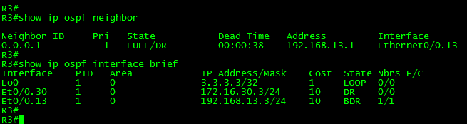
The above output show R1 is neighbor of R2, R3 and R4 respectively. The Neighbor ID column show the Router-ID corresponding to each neighbor, PRI display the neighbor reported Priority (1 – default). The State displays the state of the link (DR, BDR, DROTHER, Waiting, Point-to-Point or Point-to-Multipoint). The Address displays the neighbor’s IP address and the Interface connecting to the segment.
The show ip ospf interface brief show local summary information of the interfaces running OSPF such the Interface, Process ID (PID), the area where the interface belong, the IP address of the local interface, it’s cost, the State of the link and Neighbors Full/Count. All of the columns are self-explain but the last one. The Nbrs F/C column represents the number of neighbors on the segment in Full State vs the count of neighbors in the given segment. If there’s inconsistency, for example 1 / 2 means one neighbor on the segment has adjacency problems. Only 1 out of two is in full state.


The show ip ospf interface {interface-number} show detailed information of a given interface running OSPF.

Now, let’s examine the Link-State Database (LSDB):


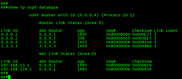
As you can see in the outputs of R1, R2, R3 and R4 LSDB, they look the same. All routers share the same information. This is because all of them are in a single area. Therefore they only have Type-1 and Type-2 LSAs. All of the routers agree on the same Designated Router (DR). As you can see on the Net Link States (Type-2 LSA) ADV router, the DR of the area is the one with RID 0.0.0.1 (R1).
The Type-1 LSA also contains information about the links reported from each network. For example, let’s take a look to the links reported from R2 (RID 0.0.0.2):

As shown in the above example, R2 advertises 3 links. The first link is reported as Stub Network and details the information of the Loopback interface of R2. The second link is also reported as a Stub Network and corresponds to the network segment 172.16.20.0/24; finally the third link is reported as Transit. Correspond to the link connecting with R1 (192.168.124.2). The Link-ID is the Router-ID of the Designated Router (DR). All three links also display its metric (Cost).
Now, let’s take a look to the Routing Table on R1:

As you can see in the output, all of the OSPF routes are coded as O – OSPF, this means they are Intra Area Routes and were generated by TYPE-1 LSAs.
Last, but not least, let’s take a look to the OSPF RIB:

The OSPF RIB serves as the primary state for OSPF route computation. Each OSPF instance has its own local Routing Information Base (RIB).
The above example shows the list of routes to be installed in the global RIB. The output is similar to the one generated by BGP.
It is noteworthy that the global routing table is updated only when routes are added, deleted or changed. This greatly reduces processing cycles and results in fewer dropped packets.
It is time to close this long post.
Thank you for visiting.